Quickstart

This guide will help you get started with DeepMIMO quickly.

Load scenario

Load a scenario and generate channels with default settings:

import deepmimo as dm

scenario = 'asu_campus_3p5'
# Download a Scenario
dm.download(scenario)

# Load to memory
dataset = dm.load(scenario)

Load will open the ray tracing scenario matrices, such as the received powers, times of arrival, and angles.

Tip

dm.download() requires an internet connection. If the scenario already exists in ./deepmimo_scenarios, the download is skipped.

Compute channels

# Generate channels with default parameters
dataset.compute_channels()

print(dataset.channels.shape)
# [n_ue, n_ue_ant, n_bs_ant, n_freqs]
# (131931, 1, 8, 1)

Tip

See the Channel Generation Examples for the default parameters and how to configure channel generation.

Visualize Dataset

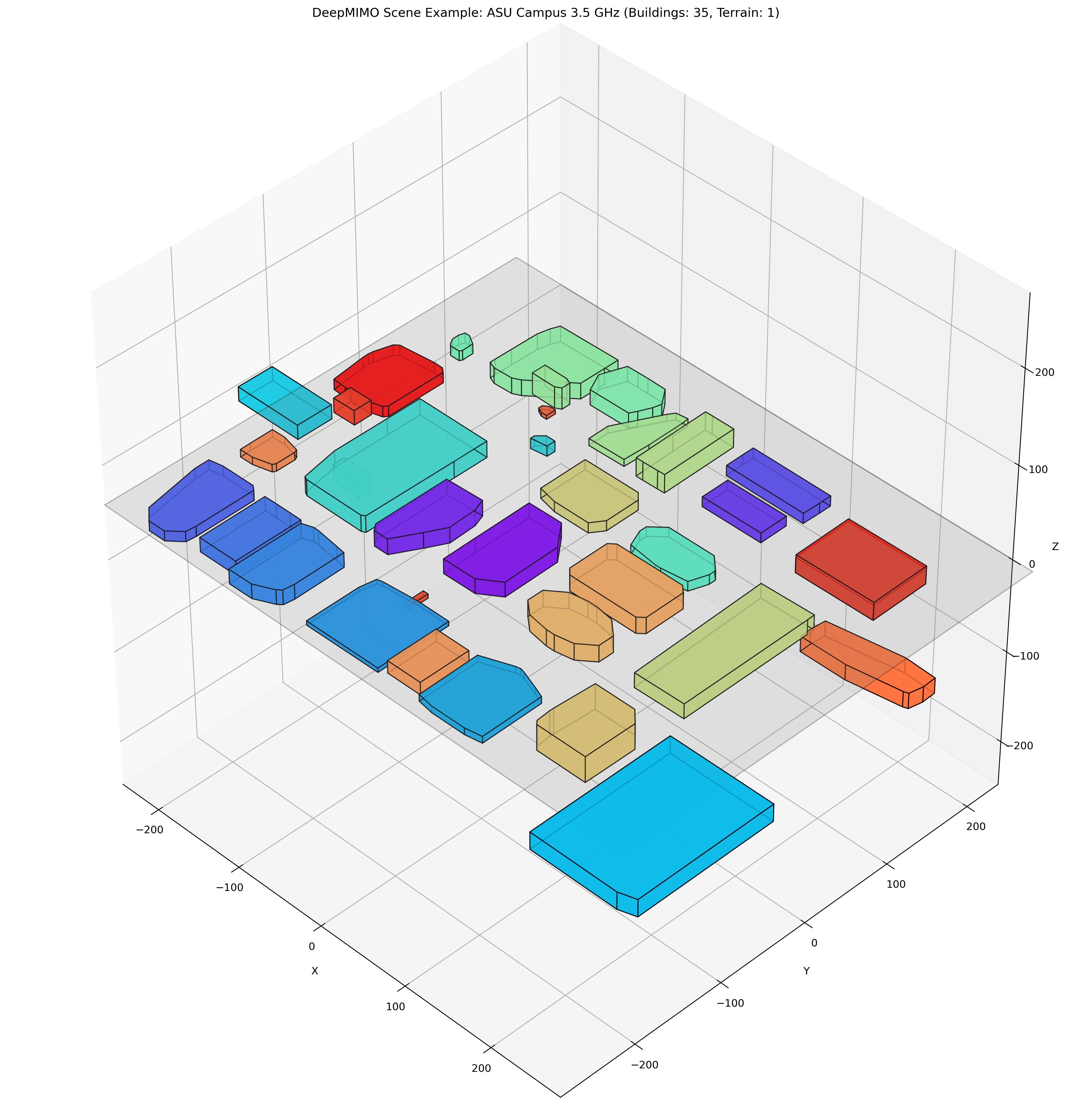
Scene

dataset.scene.plot()

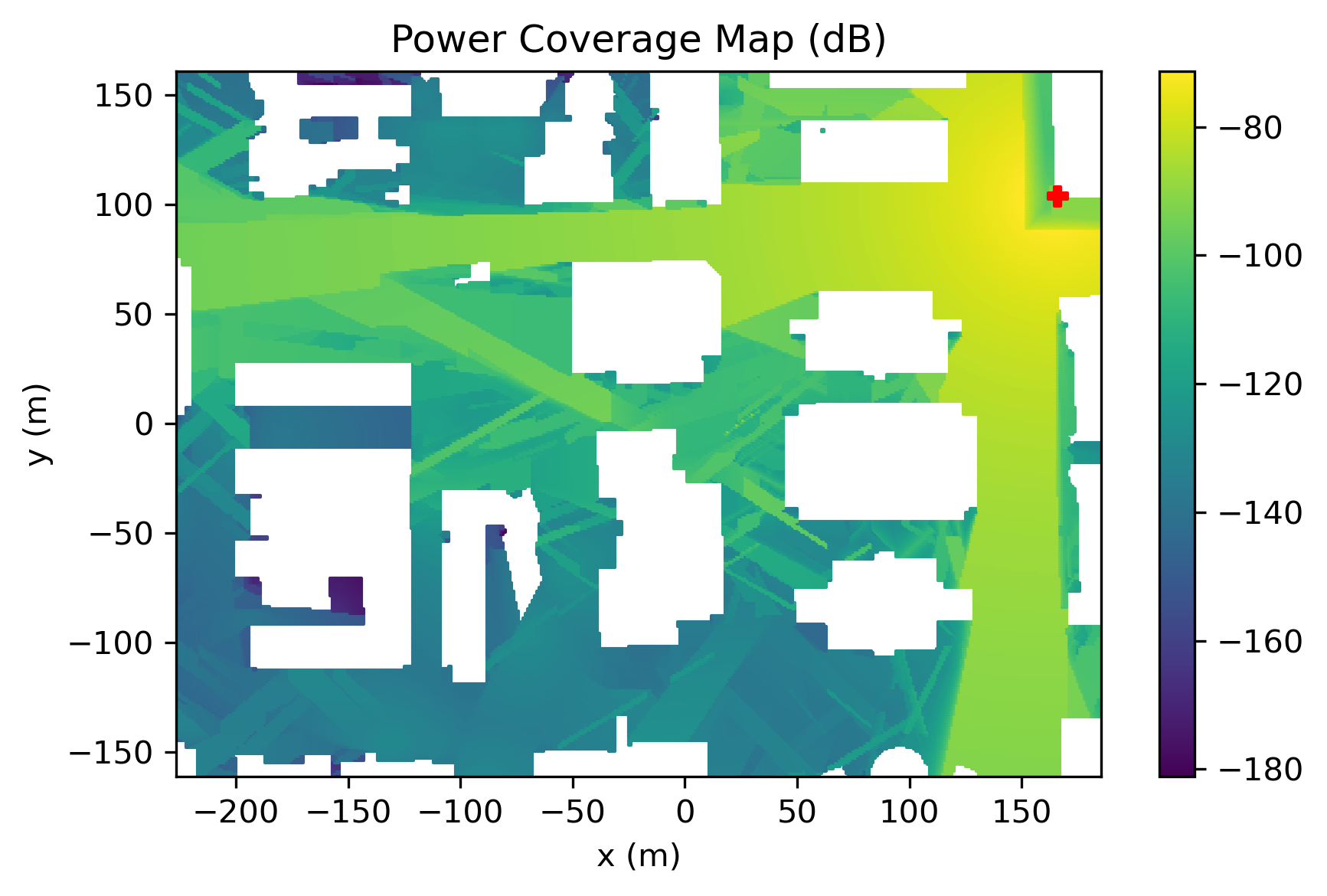
Coverage Maps

    # Plot power coverage map (power is [n_ue, n_paths])
    dataset.power.plot() # selects first path by default

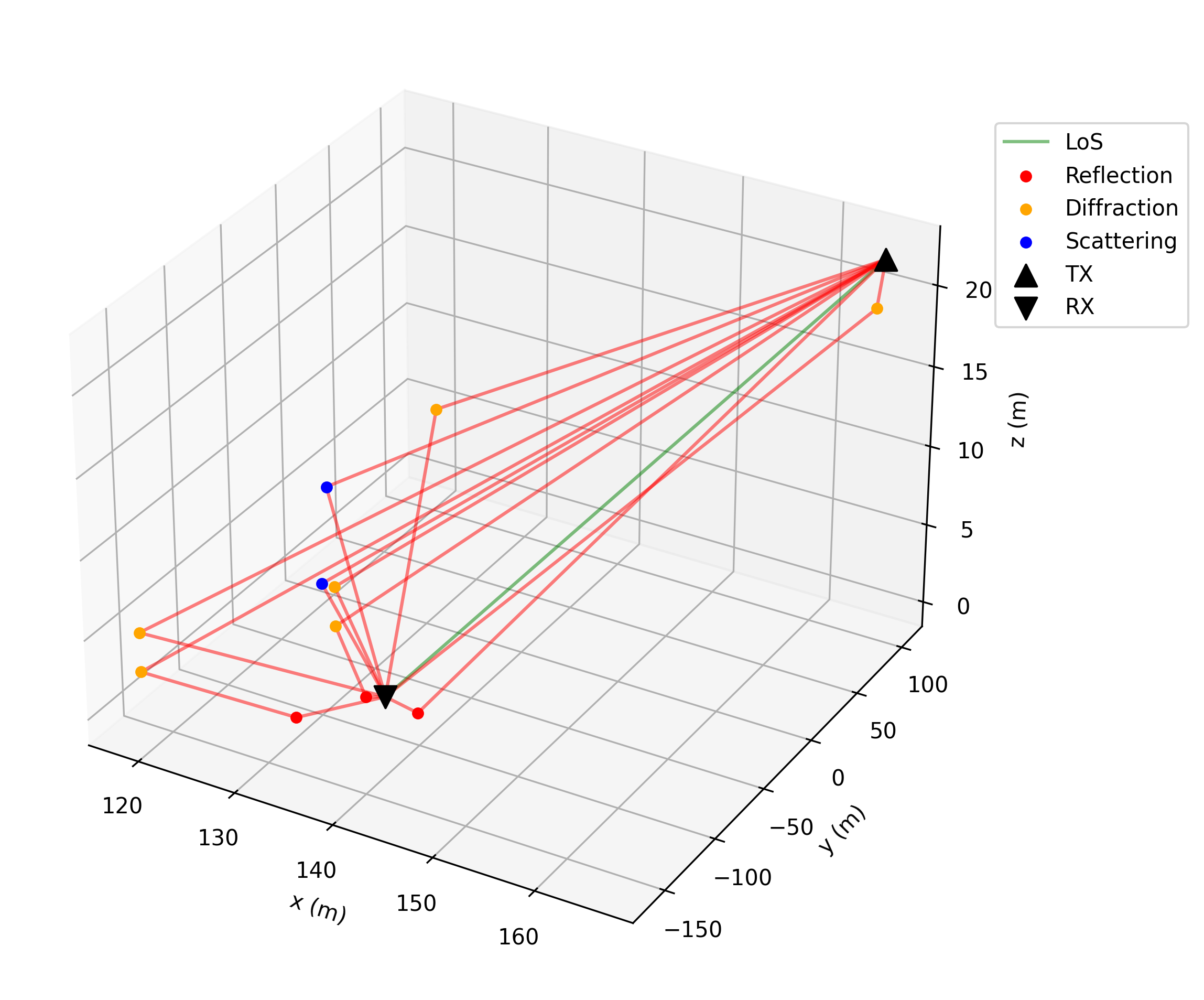
Rays

    # Plot ray paths for a user in line of sight
    los_user = np.where(dataset.los == 1)[0][2500]
    dataset.plot_rays(los_user)

Inspect Dataset

To see all matrices available in a DeepMIMO dataset, call:

    dataset.info()

This will print 3 tables, the fundamental matrices, the computed attributes, and the other dictionaries in DeepMIMO.

Fundamental Matrices

Matrix	Shape	Description
power	[num_rx, num_paths]	Tap power. Received power in dBW for each path, assuming 0 dBW transmitted power. 10*log10(|a|²), where a is the complex channel amplitude
phase	[num_rx, num_paths]	Tap phase. Phase of received signal for each path in degrees. ∠a (angle of a), where a is the complex channel amplitude
delay	[num_rx, num_paths]	Tap delay. Propagation delay for each path in seconds
aoa_az	[num_rx, num_paths]	Angle of arrival (azimuth) for each path in degrees
aoa_el	[num_rx, num_paths]	Angle of arrival (elevation) for each path in degrees
aod_az	[num_rx, num_paths]	Angle of departure (azimuth) for each path in degrees
aod_el	[num_rx, num_paths]	Angle of departure (elevation) for each path in degrees
inter	[num_rx, num_paths]	Type of interactions along each path. Codes: 0: LOS, 1: Reflection, 2: Diffraction, 3: Scattering, 4: Transmission. Code meaning: 121 -> Tx-R-D-R-Rx
inter_pos	[num_rx, num_paths, max_interactions, 3]	3D coordinates in meters of each interaction point along paths
rx_pos	[num_rx, 3]	Receiver positions in 3D coordinates in meters
tx_pos	[num_tx, 3]	Transmitter positions in 3D coordinates in meters

Computed/Derived Matrices

Matrix	Shape	Description
los	[num_rx, ]	Line of sight status for each path. 1: Direct path between TX and RX. 0: Indirect path. -1: No paths between TX and RX.
channel	[num_rx, num_rx_ant, num_tx_ant, X]	Channel matrix between TX and RX antennas. X = number of paths (time domain) or subcarriers (frequency domain)
power_linear	[num_rx, num_paths]	Linear power for each path (W)
pathloss	[num_rx, num_paths]	Pathloss for each path (dB)
distance	[num_rx, num_paths]	Distance between TX and RX for each path (m)
num_paths	[num_rx]	Number of paths for each user
inter_str	[num_rx, num_paths]	Interaction string for each path. Codes: 0:"", 1:"R", 2:"D", 3:"S", 4:"T". Example: 121 -> "RDR"
doppler	[num_rx, num_paths]	Doppler frequency shifts [Hz] for each user and path
inter_obj	[num_rx, num_paths, max_interactions]	Object ids at each interaction point

Additional Dataset Fields

Field	Description
scene	Scene parameters
materials	List of available materials and their electromagnetic properties
txrx_sets	Transmitter/receiver parameters
rt_params	Ray-tracing parameters

All these attributes can be accessed via dataset.<attribute_name>, just like we did in dataset.power.plot()

For more advanced usage and features, we recommend exploring the Examples Manual, leveraging the API reference when needed.